You know the feeling. You’re looking at a family of curves and trying to figure out what crosses them at a perfect 90-degree angle. In mathematics, we call this an orthogonal trajectory. It sounds like jargon, but it’s actually one of the most useful tools in physics and engineering.
Imagine electric fields. The lines where force flows are perpendicular to the lines of constant voltage. Or think about water flowing in a river. The path the water takes (streamlines) cuts across lines of constant speed at right angles. If you can calculate these orthogonal trajectories, you unlock how these systems work.
Here is the breakdown. No fluff. Just the math.
The Core Concept
A family of curves is defined by an equation with a parameter. Let’s call it k. Change k, and you get a different curve in that family.
Two curves are orthogonal if they intersect at right angles. In calculus, that means their slopes are negative reciprocals of each other. If one slope is m, the other is -1/m.
To find the orthogonal trajectory, you need to work backward from the original family’s slope.
Step-by-Step Calculation
-
Start with the original equation.
Let’s say you have y = f(x, k). The parameter k defines each specific curve. -
Find the derivative.
Differentiate with respect to x to get y’. This gives you the slope of any curve in the family at any point. The result will likely still contain k. -
Eliminate the parameter.
Solve the original equation for k in terms of x and y. Substitute this back into your derivative equation. Now you have y’ = g(x, y). This function tells you the slope at any point (x, y), regardless of which specific curve in the family you’re on. -
Flip the slope.
The orthogonal trajectory must have a slope that is the negative reciprocal. So, set up a new differential equation:
y’_1 = -1 / g(x, y) -
Solve the new equation.
This differential equation yields the family of orthogonal trajectories.
A Concrete Example
Let’s look at parabolas. Suppose your family of curves is:
y = kx²
First, find the derivative:
y’ = 2kx
Now, solve the original equation for k :
k = y / x²
Substitute k back into the derivative:
y’ = 2(y / x²)x
y’ = 2y / x
This is g(x, y). The slope of the parabolas at any point is 2y/x.
To find the orthogonal trajectories, flip the slope and add a negative sign:
y’_1 = -x / 2y
Now you have a separable differential equation:
2y dy = -x dx
Integrate both sides:
y² = -x²/2 + C
Rearrange:
*x²/2 + y²

Finding Orthogonal Curves Through Substitution
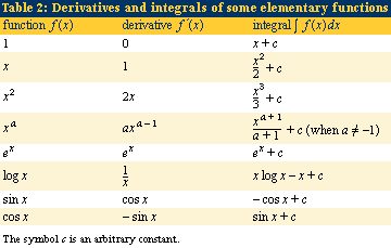
You already have the derivative formula from your analysis coursework. The trick is connecting it to the specific shape you are analyzing. Here, the relationship is defined by $k = y/x^2$.
Instead of leaving it abstract, plug that $k$ value back into the derivative equation. When you substitute and simplify, the slope $y’$ becomes $2y/x$. That is the slope of the original parabolas.
To find the curves that cut across them at right angles, you flip the slope. The orthogonal trajectory needs a gradient of $-x/2y$.
Solving that differential equation gives you a new equation entirely: $y^2 + (x^2/2) = k$.
This isn’t a parabola anymore. It’s a family of ellipses.
Look at the diagram. The red lines represent these ellipses. They intersect the original curves perpendicularly. Every time you draw a tangent on the blue curve, the red curve cuts through it at a perfect 90-degree angle. That is the geometric definition of orthogonality in action.